What are GAMs?
GAM stands for Generalized Additive Models. This is an statistical technique used to approximate smooth functions to predict a variable. In essence, smooth functions are obtained based on several cubic functions (in practice, more complex functions are utilized).
When should I use GAMs?
You could use GAMs when you do not know what is the prediction function but know the predictors (variables used to predict). Let’s take as an example the task to predict the variation fo the temperature through the day. In this example, the temperature could be predicted using the time of the day as the predictor and let GAM learn what is the the predictor function.
Example: Predicting temperature variation through the day
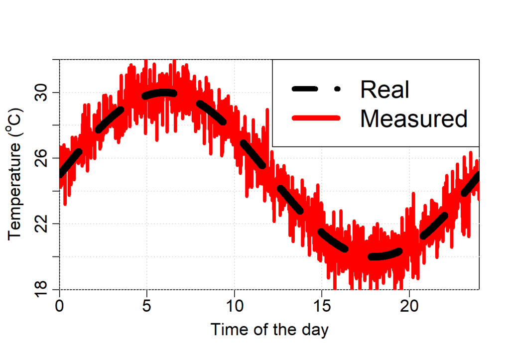
Let’s explore an artificial example in which we want to predict the temperature through the day. Let’s create our dataset
# creating time from 0 to 24 h with 1000 samples
hour = seq(0, 24, length.out = 1e3)
# creating the temperature as a fix value of 25 plus a 5 degrees oscillation
temp_real = 25 + 5*sin(hour/24*2*pi)

plot(hour, # x
     temp_real, # y
     type = 'l', # plot line
     xlab = "Time of the day", # label for x axis
     ylab = expression(paste("Temperature ("^{o},"C)", sep = "")), # label for y axis
     ylim = c(18, 32), # limits of the y axis
     lwd = 10, # line thickness
     lty = 2, # line type
     xaxs = "i", # x axis start at the lower limit of x and ends with the upper limit of x
     yaxs = "i", # y axis start at the lower limit of y and ends with the upper limit of y
     mgp=c(2.3,0.7,0), # changing the position of the labels in the axes
     cex.lab = 1.4, # increasing the label size
     cex.axis = 1.4) # increasing the number size
grid() # creating grid lines

# Let's add a measurement error
set.seed(1) # defining seed to be able to repeat the simulation
errors_measurement = rnorm(length(hour))
temp_measured = temp_real + errors_measurement

lines(hour, # x
      temp_measured, # y
      col = 'red', # line color
      lwd = 4) # line thickness

# re-ploting the real temperature so that this line stays on top of the temperature measured with errors
lines(hour, # x
      temp_real, # y
      lwd = 10, # line thickness
      lty = 2) # line type

# Creating the legend
legend('topright', # legend position
       c("Real", "Measured"), # legend text
       lwd = 7, # thickness of lines in the legend
       lty = c(2, 1), # types of lines in the legend
       col = c('black', 'red'), # color of the lines in the legend
       cex = 2) # increase legend size
Now that we have created the dataset, we can train our GAM model. To do that, we will need the R libraries mgcv and nlme.
library(mgcv) # loading the mgcv library, which also loads the nlme library

## Loading required package: nlme
## This is mgcv 1.8-31. For overview type 'help("mgcv-package")'.

# training the gam model
model.gam = gam(temp_measured # what we want to predict
                ~ # prediction formula after the ~
                  s(hour) # s(.) defines a smooth function of hour
                )
# now we look at the summary of the model
# The model was able to explain 92.3% of the deviance
summary(model.gam)
##
## Family: gaussian
## Link function: identity
##
## Formula:
## temp_measured ~ s(hour)
##
## Parametric coefficients:
##             Estimate Std. Error t value Pr(>|t|)
## (Intercept) 24.98835    0.03277   762.5   <2e-16 ***
## ---
## Signif. codes:  0 '***' 0.001 '**' 0.01 '*' 0.05 '.' 0.1 ' ' 1
##
## Approximate significance of smooth terms:
##           edf Ref.df    F p-value
## s(hour) 7.049  8.112 1451  <2e-16 ***
## ---
## Signif. codes:  0 '***' 0.001 '**' 0.01 '*' 0.05 '.' 0.1 ' ' 1
##
## R-sq.(adj) =  0.922   Deviance explained = 92.3%
## GCV = 1.0827  Scale est. = 1.074     n = 1000

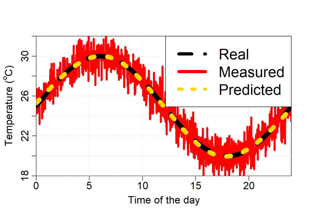
# Let's us plot the function learned by the model and compare it with the real temperature function
# obtaining predicted temperatures
temp_pred = predict(model.gam, data.frame(hour = hour))

# Let's replot the previous figure
plot(hour, # x
     temp_real, # y
     type = 'l', # plot line
     xlab = "Time of the day", # label for x axis
     ylab = expression(paste("Temperature ("^{o},"C)", sep = "")), # label for y axis
     ylim = c(18, 32), # limits of the y axis
     lwd = 10, # line thickness
     lty = 2, # line type
     xaxs = "i", # x axis start at the lower limit of x and ends with the upper limit of x
     yaxs = "i", # y axis start at the lower limit of y and ends with the upper limit of y
     mgp=c(2.3,0.7,0), # changing the position of the labels in the axes
     cex.lab = 1.4, # increasing the label size
     cex.axis = 1.4) # increasing the number size
grid() # creating grid lines

lines(hour, # x
      temp_measured, # y
      col = 'red', # line color
      lwd = 4) # line thickness

# re-ploting the real temperature so that this line stays on top of the temperature measured with errors
lines(hour, # x
      temp_real, # y
      lwd = 10, # line thickness
      lty = 2) # line type

lines(hour, # x
      temp_pred, # y
      lwd = 10, # line thickness
      lty = 3, # line type
      col = 'gold') # line color

# creating the legend
legend('topright', # legend position
       c("Real", "Measured", "Predicted"), # legend text
       lwd = 7, # thickness of lines in the legend
       lty = c(2, 1, 3), # types of lines in the legend
       col = c('black', 'red', 'gold'), # color of the lines in the legend
       cex = 2) # increase legend size
As we can see in the figure above, the temperature predicted with the GAM model is very similar to the real temperature.
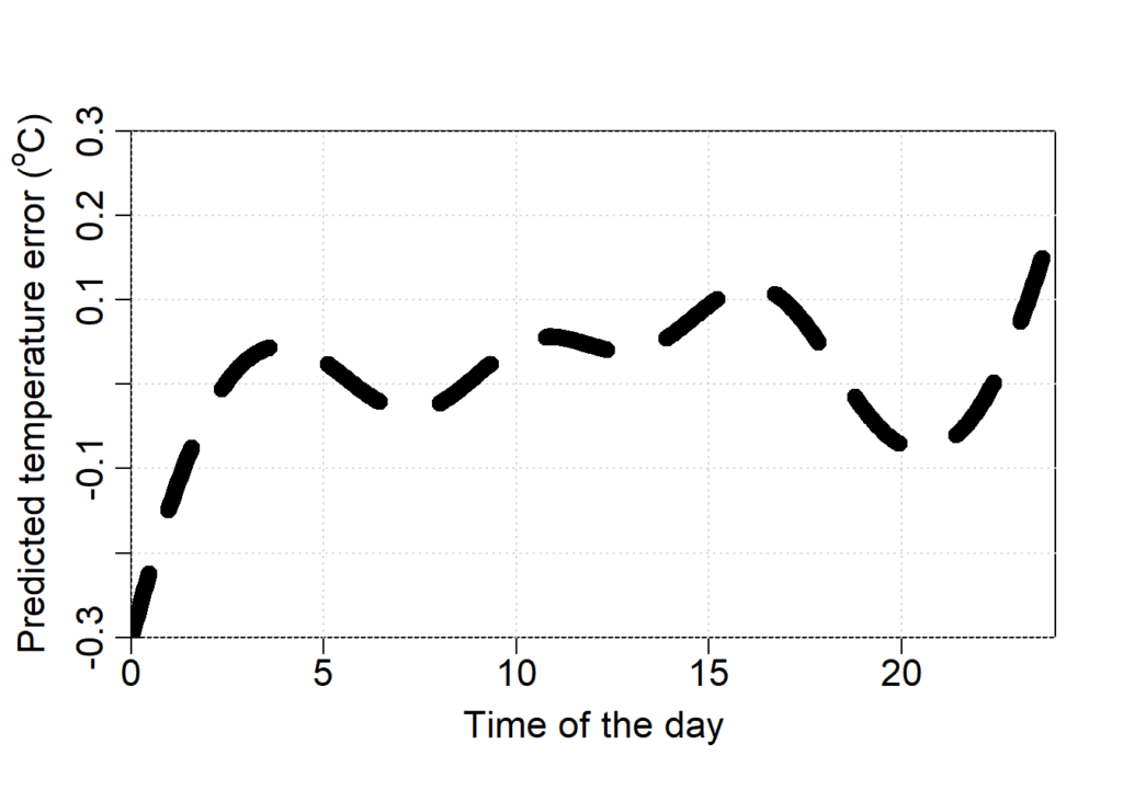
# let's plot the difference
plot(hour, # x
     temp_real - temp_pred, # y
     type = 'l', # plot line
     xlab = "Time of the day", # label for x axis
     ylab = expression(paste("Predicted temperature error ("^{o},"C)", sep = "")), # label for y axis
     ylim = c(-0.3, 0.3), # limits of the y axis
     lwd = 10, # line thickness
     lty = 2, # line type
     xaxs = "i", # x axis start at the lower limit of x and ends with the upper limit of x
     yaxs = "i", # y axis start at the lower limit of y and ends with the upper limit of y
     mgp=c(2.3,0.7,0), # changing the position of the labels in the axes
     cex.lab = 1.4, # increasing the label size
     cex.axis = 1.4) # increasing the number size
grid() # create grid lines

# I like to replot the line so that it stays above the grid:
lines(hour, # x
      temp_real - temp_pred, # y
      lwd = 10, # line thickness
      lty = 2) # line type
Where can I go to learn more?
I recommend the following:
- Book that introduces several statistical techniques in R. Zuur AF, Ieno EN, Walker NJ, Saveliev AA, Smith GM. Mixed Effects Models and Extensions in Ecology with R. Springer, New York, 2009.
- Book that describes GAM theory in R. Wood SN. Generalized Additive Models: An Introduction with R (2nd ed.). CRC Press, Boca Raton, 2017.
- Book that describes several machine learning methods. Hastie T, Tibshirani R, Friedman J. The Elements of Statistical Learning: Data Mining, Inference, and Prediction (2nd ed.). Springer, New York. 2008.
- Book that describes several machine learning methods. Efron B, Hastie T. Computer Age Statistica Inference: Algorithms, Evidence, and Data Science. Cambridge University Press, Cambridge, 2016.

